The musical chairs model, updated

It’s been about 6 months since we’ve looked at the sticky wage model, so let’s see how it’s doing:

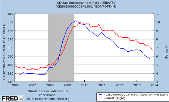
The fit seems better than ever.  To my eyes it looks like “real wages” [(nominal average hourly earnings)/(NGDP/pop)] lead unemployment by about a month or two.  That’s partly an artifact of a flaw in the St. Louis Fred graphing program. The (W/(GDP/pop)) data for Q4 is put in the October 2013 slot, whereas it should be November 2013.  If you shifted the wage series one month to the right the correlation would look even closer.

The musical chairs model does a great job of explaining both the onset of the recession, its intensity, and the slow pace of recovery.  When the blue line gets down to about 350 the recession will be over and the red line (unemployment) will be in the 5% to 5.5% range.

More M*V plus sticky wages = recovery.  It’s that simple, and always has been.

PS.  Yichuan Wang has an excellent post over at Quartz explaining why it would be foolish for the Fed to try to pop bubbles.

via:http://www.themoneyillusion.com/?p=26122&utm_source=feedburner&utm_medium=feed&utm_campaign=Feed%3A+Themoneyillusion+%28TheMoneyIllusion%29

An old monetarist interpretation of interest on money (money isn’t credit)

We can imagine a world where all central bank money is electronic money, and the central bank can alter both the quantity of money and the interest rate paid on that money, and can make Rm and Rb move by different amounts, or even in different directions, if it wants to.

To my monetarist mind, an increase in Rm increases the demand for money, and that causes an excess demand for money, just like a reduction in the supply of money causes an excess demand for money. An excess demand for money, or an excess supply of money, has macroeconomic consequences. Any change in Rb is just one symptom of those macroeconomic consequences. We would get roughly the same macroeconomic consequences even if Rb was fixed by law, or if lending money at interest was tabu.

Let’s begin by looking at this from an old monetarist perspective.  They would argue that “the money supply” is some sort of aggregate, such as M1 or M2.  Here are four ways of reducing the supply of that aggregate:

A.  Reduce the supply of base money:

1.  Do open market sales

2.  Raise the discount rate to reduce discount loans

B.  Raise the demand for base money:

3.  Raise reserve requirements

4.  Raise the interest rate paid on base money

The first two policies reduce the supply of base money, and the second two reduce the money multiplier.  All four policies reduce the monetary aggregates such as M1 and M2.  Milton Friedman would regard all four as essentially the same policy, a reduction in the supply of money.

[Because I regard money as "the base," I regard the first two as a lower supply of money and the second two as a larger demand for money.  But this is pure semantics; nothing of importance hangs on the difference between how I define 'money' and the definition used by old monetarists like Friedman.]

The interesting thing about interest on money is that it can be controlled even in a completely flexible price economy.  Recall that the only reason that changes in the monetary base lead to changes in market interest rates is that wages and prices and debt contracts are sticky.  If prices are completely flexible, as in a currency reform, a change in the money supply has no effect on interest rates. Indeed that’s even roughly true of a change in the aggregates caused by a change in the demand for base money (ignoring small “superneutrality” effect from a change in real base balances.)

A one time decrease in the money supply leads to a temporary rise in interest rates, but then when the price level adjusts interest rates fall back to their original level.

A one time increase in the interest rate on money causes a one time increase in market interest rates on bonds, but only because prices are sticky. In the long run the interest rate on money stays at its new and higher level, whereas the interest rate on bonds returns to its equilibrium level (consistent with money neutrality.)

Sticky prices make it seem like interest on money and interest on bonds are related, but that’s a cognitive illusion.  At a fundamental level a change in the interest on money is a change in the demand for the medium of account, and is a profoundly monetarist policy.  It is no different from changing the supply of base money.  In contrast, a change in the discount rate does have a direct effect on the cost of credit, and hence is a more “Keynesian” policy.  Unlike a change in the interest rate on money, which can be permanent, a change in the discount rate would lead to hyperinflation or hyperdeflation if permanent.  There is a long run Wicksellian equilibrium discount rate, whereas there is no long run Wicksellian equilibrium rate of interest on money.  The central bank is the monopoly supplier of base money and can attach any (reasonable) tax or subsidy it wishes, even in the long run.

Money is not credit.  That’s the whole point of this post.

Update:  Obviously the interest on money should not exceed the interest on bonds

via:http://www.themoneyillusion.com/?p=26133

If it’s an identity does that mean I’m right?

My musical chairs model of the economy assumes nominal hourly wages are sticky. In that case fluctuations in NGDP may be highly correlated with changes in the unemployment rate.  Arnold Kling doesn’t like the empirical evidence I found in support of the model:

Scott is fond of saying, “Never reason from a price change.” I say, “Never draw a behavioral inference from an identity.”

I think Arnold knows it’s not an identity.  If you graphed MV and PY, you’d observe only one line, as the two lines would perfectly overlap.  In the graph I presented the two lines were correlated but far from perfectly correlated.  So it’s no identity. I’d guess the gaps would be far larger in many other countries, such as Zimbabwe.

A better argument would be that the correlation doesn’t prove that causation goes from NGDP to unemployment.  After all, changes in NGDP could cause changes in hourly nominal wage rates, leaving unemployment roughly unchanged.  In that case the correlation I found would be spurious. If I left the impression that the correlation proved nominal wages were sticky that would have been a “behavioral inference,” and hence a mistake.  What I tried to do was assume nominal wages are sticky (as they obviously are), and then show the effect of NGDP shocks in a world where nominal wages are sticky.

My musical chair model doesn’t have the “microfoundations” that have been fashionable since the 1980s.  But which model with microfoundations can outperform the musical chairs model?  Indeed let’s make the claim more policy-oriented.  I claim that fluctuations in predicted future NGDP relative to the trend line strongly correlate with changes in future unemployment.  And of course NGDP futures prices are 100% controllable by the monetary authority.

There is no NGDP futures market?  You can’t use that against my claim as I’ve been advocating such a market since 1986.  It’s an embarrassment to the economics profession that this market doesn’t exist (yet.)

So yes, it sort of seems like a tautology, but perhaps that’s because I’m right.

PS.  Imagine one of the great controversies in physics (say string theory) could be settled with a particle accelerator that cost $500,000 to build.  But the physics profession was too lazy to ask the NSF for the money.  Replace string theory with the debate over demand-side vs. RBC models and you have described economics circa 2014.

via:http://www.themoneyillusion.com/?p=26148&utm_source=feedburner&utm_medium=feed&utm_campaign=Feed%3A+Themoneyillusion+%28TheMoneyIllusion%29

Daniel Thornton on QE

The analysis presented here suggests that QE had little or no effect in reducing long-term yields relative to what they would have otherwise been.² If QE did not significantly reduce long-term yields relative to what they would have otherwise been, it cannot have increased output or employment either.

I’m old enough to recall when the St Louis Fed had monetarist leanings.  A monetarist would immediately reply that interest rates are a lousy indicator of the stance of monetary policy.  But this statement isn’t even consistent with New Keynesian models.  After all, QE could easily raise the Wicksellian equilibrium interest rate in a NK model, and hence boost AD even if actual interest rates did not change.  Thus the term ‘cannot’ is way too strong.  What if the Fed had done Zimbabwe-style QE.  Would you expect interest rates to fall?  Would NGDP growth rise?

I’m also puzzled as to why he looks at time series data and not market reactions to policy announcements.

Elsewhere Thornton acknowledges that there are other possible mechanisms:

Another possibility is that other countries experienced a greater output decline relative to that of the United States, which caused their yields to decline compared with the United States. The second chart shows the gross domestic product (GDP) growth rates of Canada, France, Germany, the United States, and the United Kingdom since 2005. The GDP growth patterns of four of the five countries have been similar since the fourth quarter of 2008; the sole exception is France, whose growth declined more. Hence, it appears unlikely that divergent growth rates could account for the lack of support for QE.

Lots of puzzles here.  Surely US growth has exceeded British growth by a wide margin.  In any case, Britain also did lots of QE, so why make this comparison? Germany and France don’t even have their own monetary policies; they are part of the eurozone. And growth in the eurozone has been far below US levels, presumably due to the ECB’s unwillingness to be as expansionary as the Fed. Indeed they raised interest rates twice in 2011.

PS.  Off topic, but notice all the chatter about how unemployment is not a useful policy guide for the Fed.  Who argued the Evan’s rule should have been based on levels of NGDP.  I hate love to say I told you so . . .

via:http://www.themoneyillusion.com/?p=26159&utm_source=feedburner&utm_medium=feed&utm_campaign=Feed%3A+Themoneyillusion+%28TheMoneyIllusion%29

I predict that Steve Keen will eventually look

. . . without actually being correct.

For years I’ve pointed out that whereas the huge house price run-up in the US was reversed after 2006, house prices in Britain, Canada, Australia, and New Zealand remained at lofty levels, after a similar rise in prices.  Indeed Australian house prices moved still higher.

Commenters kept insisting “you just wait, the Australian housing bubble will burst one of these days.”  Australian economist Steve Keen was so sure the bubble would burst that he bet his reputation on it:

Mr Keen is a long time bear on Australian house prices, who famously lost a bet with an economist at Macquarie Bank in 2008 over his claim that prices would soon reverse sharply. Two years later he walked 225km from parliament house to Mount Kosciuszko wearing a T-shirt saying “I was hopelessly wrong on house prices – ask me how” to honour the wager.

That’s why I like Aussies, they have an honesty that is increasingly rare in our world.  Now Australian housing prices are soaring higher again.  Is it a bubble on top of a bubble?

And in Australia too, foreign buyers, together with cheap money and supply constraints, have helped push up house prices, prompting some commentators to warn of an emerging housing bubble in some of the country’s bigger cities.

(Read more: Are fears of an Australian housing bubble overblown?)

Prices in Sydney jumped 15.1 percent last year, pushing the median house price to A$763,169. In Melbourne and Perth, property prices increased 8 percent, according to Australian Property Monitors, an information provider to the banking and property industries.

“I think we are seeing the creation of a spectacular bubble on top of a spectacular property bubble,” says Steve Keen, a professor of economics and author of a blog called Debtwatch.

Keep in mind that although Australia has 23 million people (same as Shanghai) squeezed into an area the size of the continental US, almost all of them live in “the country’s bigger cities,” which feature California-style restrictive zoning.  So prices may or may not stay high.

Since I’ve been proved right on the fact that the earlier run-up in prices was not a bubble, I’ll take my chips from the table and go home.  No further predictions; I’ve proved my point that “bubbles” are not a useful concept for Australia.  OK, just one more prediction.  I predict that if Steve Keen continues to predict bubbles in Australia there will come a time when it will look like he is correct, and he’ll be feted as the greatest seer since Nouriel Roubini.

Of course he won’t have been correct about there being a bubble, as bubbles don’t exist.  Asset markets move up and down unpredictably.  That’s the whole point of the EMH.  Ex ante there was no way of knowing in 2006 that Australian prices would keep going up while US prices would reverse and fall.  It could have been the other way around.

BTW.  Australia’s been running big current account deficits for decades, and they can continue doing so for many centuries to come.  (When I lived there in 1991 one pundit told me that Australia had a bleak future because of its CA deficits.) Australia gets some cars and TVs built with Chinese labor, and China gets some retirement condos on the Gold Coast built with Australian labor. Believe it or not economists call that sort of mutually beneficial business deal a “deficit.”  I’m not kidding. Don’t be fooled by words, focus on reality.

via:http://www.themoneyillusion.com/?p=26140&utm_source=feedburner&utm_medium=feed&utm_campaign=Feed%3A+Themoneyillusion+%28TheMoneyIllusion%29

My talks in Bristol this Wed and London this Thurs

1. Causality and statistical learning (Wed 12 Feb 2014, 16:00, at University of Bristol):

Causal inference is central to the social and biomedical sciences. There are unresolved debates about the meaning of causality and the methods that should be used to measure it. As a statistician, I am trained to say that randomized experiments are a gold standard, yet I have spent almost all my applied career analyzing observational data. In this talk we shall consider various approaches to causal reasoning from the perspective of an applied statistician who recognizes the importance of causal identification, yet must learn from available information.

This is a good one. They laughed their asses off when I did it in Ann Arbor. But it has serious stuff too. As George Carlin (or, for that matter, John or Brad) might say, it’s funny because it’s true. Here are some old slides, but I plan to mix in a bit of new material.

2. Theoretical Statistics is the Theory of Applied Statistics (Thurs 13 Feb 2014, 17:00, at Imperial College London):

The audience will get to vote on which of the following talks they’d like to hear:
- Choices in statistical graphics
- Little Data: How traditional statistical ideas remain relevant in a big-data world
- Weakly informative priors

Actually, I’d be happy to give any of my prepared talks (except I don’t want to repeat the talk from Bristol). What happened was that I was paranoid on what to speak about. On one hand, the applied stuff is of broadest interest, and even theory people like to hear about what’s going on in American politics. On the other hand, I don’t want to get the reputation as a softie, and I do do technical things from time to time. So I thought I’d throw the choice at the audience. That way, if they pick something technical, I know they actually want to hear it, and if they pick something softer, at least it’s clear that it’s their choice. All three of the above are fine (really, I should add some material to talks #2 and 3 above, maybe I’ll do some of that on the train).

via:http://andrewgelman.com/2014/02/11/talks-bristol-wed-london-thurs/

How to think about “identifiability” in Bayesian inference?

We had some questions on the Stan list regarding identification. The topic arose because people were fitting models with improper posterior distributions, the kind of model where there’s a ridge in the likelihood and the parameters are not otherwise constrained.

I tried to help by writing something on Bayesian identifiability for the Stan list. Then Ben Goodrich came along and cleaned up what I wrote. I think this might be of interest to many of you so I’ll repeat the discussion here.

Here’s what I wrote:

Identification is actually a tricky concept and is not so clearly defined. In the broadest sense, a Bayesian model is identified if the posterior distribution is proper. Then one can do Bayesian inference and that’s that. No need to require a finite variance or even a finite mean, all that’s needed is a finite integral of the probability distribution.

That said, there are some reasons why a stronger definition can be useful:

1. Weak identification. Suppose that, with reasonable data, you’d have a posterior with a sd of 1 (or that order of magnitude). But you have sparse data or collinearity or whatever, and so you have some dimension in your posterior that’s really flat, some “ridge” with a sd of 1000. Then it makes sense to say that this parameter or linear combination of parameters is only weakly identified. Or one can say that it’s identified from the prior but not the likelihood.

If we wanted to make this concept of “weak identification” more formal, we could stipulate that the model is expressed in terms of some hyperparameter A which is set to a large value, and that weak identifiability corresponds to nonidentifiability when A -> infinity.

Even there, though, some tricky cases arise. For example, suppose your model includes a parameter p that is defined on [0,1] and is given a Beta(2,2) prior, and suppose the data don’t tell us anything about p, so that our posterior is also Beta(2,2). That sounds nonidentified to me, but it does have a finite integral.

2. Aliasing. Consider an item response model or ideal point model or mixture model where the direction or labeling is unspecified. Then you can have 2 or 4 or K! different reflections of the posterior. Even if all priors are proper, so the full posterior is proper, it contains all these copies so this labeling is not identified in any real sense.

Here, and in general, identification depends not just on the model but also on the data. So, strictly speaking, one should not talk about an “identifiable model” but rather an ‘identifiable fitted model” or “identifiable parameters” within a fitted model.

Ben supplied some more perspective. First, in reaction to my definition that a Bayesian model is identified if the posterior distribution is proper, Ben said he agreed, but in that case “what good is the word ‘identified’? If the posterior distribution is improper, then there is no Bayesian inference.”

I agree with Ben, indeed the concept of identification is less important in the Bayesian world than elsewhere. For a Bayesian, it’s generally not a black-and-white issue (“identified” or “not identified”) but rather shades of gray: considering some parameter or quantity of inference (qoi), how much information is supplied by the data. This suggests some sort of continuous measure of identification: for any qoi, corresponding to how far the posterior, p(qoi|y), is from the prior, p(qoi).

Ben continues:

I agree that a lot of people use the word identification without defining what they mean, but there are no shortage of definitions out there. However, I’m not sure that identification is that helpful a concept for the practical problems we are trying to solve here when providing recommendations on how users should write .stan files.

I think many if not most people that think about identification rigorously have in mind a concept that is pre-statistical. So, for them it is going to sound weird to associate “identification” with problems that arise with a particular sample or a particular computational approach. In economics, the idea of identification of a parameter goes back at least to the Cowles Commission guys, such as in the first couple of papers here.

In causal inference, the idea of identification of an average causal effect is a property of a DAG in Pearl’s stuff.

I’d like to hold fast to the idea that identification, to the extent it means anything, must be defined as a function of model + data, not just of the model. Sure, with a probability model, you can say that asymptotically you’ll get identification, but asymptotically we’re all dead, and in the meantime we have sparseness and separation and all sorts of other issues.

Ben also had some things to say about my casual use of the term “weak identification” to refer to cases where the model is so weak as to provide very little information about a qoi. Here’s Ben:

Here again we are running into the problem of other people associating the phrase “weak identification” with a different thing (usually instrumental variable models where the instruments are weak predictors of the variable they are instrumenting for). This paper basically is interested in situations where some parameter is not identified iff another parameter is zero. And then they drift the population toward that zero.

Ben thought my above “A -> infinity” definition was kinda OK but he recommended I not use the term “weak identifiability” which has already been taken. Maybe better for us to go with some measure of the information provided in the shift from prior to posterior. I actually had some of this in my Ph.D. thesis . . .

Regarding my example where the data provide no information on the parameter p defined on (0,1), Ben writes:

Do you mean that a particular sample doesn’t tell us anything about p or that data are incapable of telling us anything about p? In addition, I think it is helpful to distinguish between situations where
(a) There is a unique maximum likelihood estimator (perhaps with probability 1)
(b) There is not a unique maximum likelihood estimator but the likelihood is not flat everywhere with respect to a parameter proposal
(c ) The likelihood is flat everywhere with respect to a parameter proposal
What bothers me about some notion of “computational identifiability” is that a Stan user may be in situation 1 but through some combination of weird priors, bad starting values, too few iterations, finite-precision, particular choice of metric, maladaptation, and / or bad luck can’t get one or more chains to converge to the stationary distribution of the parameters. That’s a practical problem that Stan users face, but I don’t think many people would consider it to be an identification problem.

Maybe something that is somewhat unique to Stan is the idea of identified in the constrained parameter space but not identified in the unconstrained parameter space like we have with uniform sampling on the unit sphere.

Regarding Ben’s remarks above, I don’t really care if there’s a unique maximum likelihood estimator or anything like that. I mean, sure, point estimates do come up in some settings of approximate inference, but I wouldn’t want them to be central to any of our definitions.

Regarding the question of whether identification is defined conditional on the data as well as the model, Ben writes:

Certainly, whether you have computational problems depends on the data, among other things. But to say that identification depends on the data goes against the conventional usage where identification is pre-statistical so we need to think about whether it would be more effective to try to redefine identification or to use other phrases to describe the problems we are trying to overcome.

Hmm, maybe so. Again, this might motivate the quantitative measure of information. For Bayesians, “information” sounds better than “identification” anyway.

Finally, recall that the discussion all started because people were having problems running Stan with improper posteriors or with models with nearly flat priors and where certain parameters were not identified by the data alone. Here’s Ben’s summary of the situation, to best help users:

We should start with the practical Stan advice and avoid the word identifiability. The basic question we are trying to address is “What are the situations where the posterior is proper, but Stan nevertheless has trouble sampling from that posterior?” There is not much to say about improper posteriors, except that you basically can’t do Bayesian inference. Although Stan can optimize a log-likelihood function, everybody doing so should know that you can’t do maximum likelihood inference without a unique maximum. Then, there are a few things that are problematic such as long ridges, multiple modes (even if they are not exactly the same height), label switches and reflections, densities that approach infinity at some point(s), densities that are not differentiable, discontinuities, integerizing a continuous variable, good in the constrained space vs. bad in the constrained space, etc. And then we can suggest what to do about each of these specific things without trying to squeeze them under the umbrella of identifiability.

And that seems like as good as any place to end it. Now I hope someone can get the economists to chill out about identifiability as well. . .

via:http://andrewgelman.com/2014/02/12/think-identifiability-bayesian-inference/

Stopping rules and Bayesian analysis

I happened to receive two questions about stopping rules on the same day.

First, from Tom Cunningham:

I’ve been arguing with my colleagues about whether the stopping rule is relevant (a presenter disclosed that he went out to collect more data because the first experiment didn’t get significant results) — and I believe you have some qualifications to the Bayesian irrelevance argument but I don’t properly understand them.

Then, from Benjamin Kay:

I have a question that may be of interest for your blog. I was reading about the early history of AIDS and learned that the the trial of AZT was ended early because it was so effective:

The trial reported in the New England Journal of medicine, had produced a dramatic result. Before the planned 24 week duration of the study, after a mean period of participation of about 120 days, nineteen participants receiving placebo had died while there was only a single death among those receiving AZT. This appeared to be a momentous breakthrough and accordingly there was no restraint at all in reporting the result; prominent researchers triumphantly proclaimed the drug to be “a ray of hope” and “a light at the end of the tunnel”. Because of this dramatic effect, the placebo arm of the study was discontinued and all participants offered 1500mg of AZT daily.

It is my understanding that this is reasonably common when they do drug studies on humans. If the treatment is much, much better than the control it is considered unethical to continue the planned study and they end it early.

I certainly understand the sentiment behind that. However, I know that it isn’t kosher to keep adding time or sample to an experiment until you find a result, and isn’t this a bit like that? Shouldn’t we expect regression to the mean and all that?

When two people come to me with a question, I get the impression it’s worth answering. So here goes:

First, we discuss stopping rules in section 6.3 (the example on pages 147-148), section 8.5, and exercise 8.15 of BDA3. The short answer is that the stopping rule enters Bayesian data analysis in two places: inference and model checking:

1. For inference, the key is that the stopping rule is only ignorable if time is included in the model. To put it another way, treatment effects (or whatever it is that you’re measuring) can vary over time, and that possibility should be allowed for in your model, if you’re using a data-dependent stopping rule. To put it yet another way, if you use a data-dependent stopping rule and don’t allow for possible time trends in your outcome, then your analysis will not be robust to failures with that assumption.

2. For model checking, the key is that if you’re comparing observed data to hypothetical replications under the model (for example, using a p-value), these hypothetical replications depend on the design of your data collection. If you use a data-dependent stopping rule, this should be included in your data model, otherwise your p-value isn’t what it claims to be.

Next, my response to Benjamin Kay’s question about AZT:

For the Bayesian analysis, it is actually kosher “to keep adding time or sample to an experiment until you find a result.” As noted above, you do lose some robustness but, hey, there are tradeoffs in life, and robustness isn’t the only important thing out there. Beyond that, I do think there should be ways to monitor treatments that have already been approved, so that if problems show up, somebody becomes aware of them as soon as possible.

P.S. I know that some people are bothered by the idea that you can keep adding time or sample to an experiment until you find a result. But, really, it doesn’t bother me one bit. Let me illustrate with a simple example. Suppose you’re studying some treatment that has a tiny effect, say 0.01 on some scale in which an effect of 1.0 would be large. And suppose there’s a lot of variability, so if you do a preregistered study you’re unlikely to get anything approaching certainty. But if you do a very careful study (so as to minimize variation) or a very large study (to get that magic 1/sqrt(n)), you’ll get a small enough confidence interval to have high certainty about the sign of the effect. So, from going from high sigma and low n, to low sigma and high n, you’ve “adding time or sample to an experiment” and you “found a result.” See what I did there? OK, this particular plan (measure carefully and get a huge sample size) is chosen ahead of time, it doesn’t involve waiting until the confidence interval excludes zero. But so what? The point is that by manipulating my experimental conditions I can change the probability of getting a conclusive result. That doesn’t bother me. In any case, when it comes to decision making, I wouldn’t use “Does the 95% interval exclude zero?” as a decision rule. That’s not Bayesian at all.

It seems to me that problems with data-based stopping and Bayesian analysis (other than the two issues I noted above) arise only because people are mixing Bayesian inference with non-Bayesian decision making. Which is fair enough—people apply these sorts of mixed methods all the time—but in that case I prefer to see the problem as arising from the non-Bayesian decision rule, not from the stopping rule or the Bayesian inference.

via:http://andrewgelman.com/2014/02/13/stopping-rules-bayesian-analysis/

CmdStan and RStan v2.2.0

The Stan Development Team is happy to announce CmdStan and RStan v2.2.0.

PyStan will follow shortly.

This is a minor release with a mix of bug fixes and features. For a full list of changes, please see the v2.2.0 milestone on stan-dev/stan’s issue tracker. Some of the bug fixes and issues are listed below.

Bug Fixes

• increment_log_prob is now vectorized and compiles with vector arguments
• multinomial random number generator used the wrong size for the return value
• fixed memory leaks in auto-diff implementation
• variables can start with the prefix ‘inf’
• fixed parameter output order for arrays when using optimization
• RStan compatibility issue with latest Rcpp 0.11.0

Features

• suppress command line output with refresh <= 0
• added 1 to treedepth to match usual definition of treedepth
• added distance, squared_distance, diag_pre_multiply, diag_pre_multiply to Stan modeling lnaguage
• added a ‘fixed_param’ sampler for use with the generated quantities block

For more information and download links, visit Stan’s webpage: http://mc-stan.org

– Stan Development Team

via:http://andrewgelman.com/2014/02/13/cmdstan-v2-2-0/

The popularity of certain baby names is falling off the clifffffffffffff

I was looking at baby name data last night and I stumbled upon something curious. I follow the baby names blog occasionally but not regularly, so I’m not sure if it’s been noticed before. Let me present it like this: Take the statement…

Of the top 100 boys and top 100 girls names, only ___% contain the letter __.

I’m using the SSA baby names page, so that’s U.S. births, and I’m looking at the decade of 2000-2009 (so kids currently aged 4 to 13). Which letters would you expect to have the lowest rate of occurrence?

As expected, the lowest score is for Q, which appears zero times. (Jacqueline ranks #104 for girls.) It’s the second lowest that surprised me.

(… You can pause and try to guess now. Spoilers to follow.)

Of the other big-point Scrabble letters, Z appears in four names (Elizabeth, Zachary, Mackenzie, Zoe) and X in six, of which five are closely related (Alexis, Alexander, Alexandra, Alexa, Alex, Xavier). J is heavily overrepresented, especially as an initial letter, with 29 names. Former powerhouse names James and John have fallen a bit lately, to #17 and #18, but Jacob and Joshua have surged past them and rank #1 and #3 in the 2000s.

Lower than any of those is a letter I normally think of as a middle-range (ranking 15 in the ETAOIN SHRDLU): F occurs in only three top 100 names, all girls (Jennifer, Faith, Sofia). It’s not that F names never existed. Names like Frank, Jeff, Fred, and Cliff used to be common, but they have all greatly declined in recent years.

And it’s not just that F has the fewest names (other than Q), but they rank lower as well. Jennifer, which was #1 in the 1970s and #2 in the 1980s, is down to #39 in the 2000s. All the other letters have at least one high-ranking name. For X, Alexis is #11 for girls and Alexander is #13 for boys. For Z, Elizabeth is #9. (Zachary was #16 in the 1990s, down to #27 in the 200s.)

The other two letters that occur in fewer than 10 names are P and W. W has five names, all boys, but three of them rank in the top ten (Matthew #4, Andrew #7, William #10, Owen, Wyatt). P has six names, with two in the top ten (Christopher #6, Joseph #9, Sophia #13, Stephanie, Paige, Patrick).

The P list provides an interesting clue to what may have happened to F. The top four P names all use PH to make the F sound. Perhaps part of the reason that the F has disappeared from names is that in names people prefer to spell the F sound as PH. (But then if so, that would leave P as underrepresented instead.)

But counting the number of names in the top 100 is a crude way of looking at this. What I really want is

Among [all/male/female] births in [year], ___% were given a name that [contains/starts with/ends with] [text string].

so that I can input the bracketed variables and get the % as output. Then I’d run that for each single letter for the past 20 years or so, and then I’d draw a graph plotting each letter across time so I could see where the letter rank relative to each other and how they’ve trended.

SSA provides complete comma-delimited text files for each year showing number of births for every name with 5 or more occurrences, so the data is available.

I suppose I could do it in Excel, but it would be slow and laborious. I imagine you stat people have tools (and practice) that could do it much more efficiently and thoroughly.

I don’t know if this interests you enough to spend any time playing around with it. Maybe if you have a student looking for an exercise to play with you could put it out there.

P.S. Other fun fact: A’s dominance of names seems to be increasing. I didn’t count all 100 for the 2000s, but in the top 10 male and female names for 2012, 19 of 20 contain the letter A. Next is I with 12.

I asked if you could the F in Cliff twice? I sort of think it should count double, actually, as it represents that much more exposure to the letter.

Ubs replied:

No, I wouldn’t. I suppose you could do it either way, but I’m thinking in terms of the name contains the letter or it doesn’t, not how many times.

The difference is more obvious when you think of higher frequencies. Like it would be interesting to say “75% of all boys born in 2012 have an A in their name”, but not so much to say, “In the first names of the 2,000,000 boys born in 2012, the letter A occurs 1,600,000 times”. The latter method only compares letters to other letters. The former compares letters to people, which is more interesting to me.

Or to put it another way, I’m not interested in letter frequency per se across the limited text corpus of baby names. I’m interested in the probability that a person you meet will have a certain letter somewhere in his name. So if there were a trend for names to become longer, in my conception all the frequencies would go up as a result, whereas in the other conception they’re essentially relative frequencies so it would be zero sum.

In any case, in response to Ubs’s original question, this looks like a job for perl or whatever the cool kids are using these days. Python? I dunno. I bet one of our readers could download the data, crunch the numbers, and make a cool graph, all during the time it will take me to write my next blog post.

via:http://andrewgelman.com/2014/02/14/popularity-certain-baby-names-falling-clifffffffffffff/

Prediction Comes True, Belatedly

A year and a half ago, I predicted "I suspect that ... in less than a year major carriers will have to reduce their monthly cellular charges to be much closer to Straight Talk [the Walmart cell services plan]." (emphasis added)

I'm not sure when T-Mobile cut their prices, but AT&T did not, until now.
via:http://caseymulligan.blogspot.in/2014/02/predictions-comes-true-belatedly.html

CBO moves toward my estimate

I have predicted that the ACA would contract the labor market about 3 percent. Maybe more, maybe less, but that was my best guess. I continue to work on it.

Meanwhile, CBO was saying 0.5 percent, and my critics (rather than giving an economic argument), point to the "nonpartisan CBO's" estimate as proof that I am out on the fringes.

Today CBO revised -- tripled -- its estimate to 1.5 percent. They still have a bit of the economics wrong, but it is a major step that they now acknowledge most (but not all) of the incentives that have been identified, and their analysis is vastly closer to mine now.

CBO should be credited for honestly re-assessing perhaps their most cited estimate ever. I imagine that it might have been tempting to stick with the original. But CBO Director Elmendorf was one of my teachers in college, and knowing him I expected that a better estimate would be forthcoming as research increasingly clarified what was missing in the original.

I also give the CBO credit for never falling into the trap that ACA = Romneycare, ergo the ACA's labor market effects are minimal. HHS will be asked to answer the CBO's revision, and I guarantee you that they will tempt the rest of America to fall in the trap.

The real problem for America was not the CBO estimate but that such a sweeping law was passed before the best economists in the nation could digest the incentives and unintended costs that it contained.

via:http://caseymulligan.blogspot.in/2014/02/cbo-moves-toward-my-estimate.html

Remember what the President said about the ACA and the Labor Market

By default, if the supply of labor decreases, the demand will increase. And since this market has consistently had an excess supply (for the last 10-15 years), then there will be NO decrease in the amount of jobs offered. Perhaps you have other concerns, but this slack MUST be eliminated if you are truly a proponent of efficient markets. And as the demand increases, so will the buyer's price offered to labor's sellers, i.e. wages will rise. If there is a downside to any of this, they do not in any way redound to the job seekers; at least not until the unemployment rate drops to the 4% range, and the involuntary labor participation rate decreased considerably from it's current level. We are quite a ways away from either of those occurrences. Though I don't believe my analysis can be challenged, I am interested to hear your refutation.
via:http://caseymulligan.blogspot.in/2014/02/remember-what-president-said-about-aca.html

Cutler and Pollack are not with the White House Economists

Both Cutler and Pollack got the wrong impression that I called them dishonest. I did not write the WSJ article and did not call them dishonest. I told the WSJ interviewer that the 2011 letter authors and signers were unaware of the disincentives in the ACA:

there was "a general lack of awareness" and economists simply didn't realize everything that government was doing to undermine incentives for work. "You have to dig into it and see it,"

Regarding the White House economists and their allies this week (neither Cutler nor Pollack are in that group. Hardly any of the letter signers are either) who now praise the market-contracting/drudgery-avoiding attributes of their policies, I said "it looks like they're trying to leverage the lack of economic education in their audience by making these sorts of points."

To be clear, Cutler and Pollack did not and are not trying to leverage the lack of economic education ... That's Furman, Krugman, etc.

via:http://caseymulligan.blogspot.in/2014/02/cutler-and-pollack-are-not-with-white.html

The ACA and wages

The ACA reduces hourly employer cost in at least 3 ways:

(1) employer penalty. I doubt the national accountants will count this as employee comp, so it will lower measured employer cost even if it raises marg prod of labor

(2) productivity. the aca changes the allocation of factors to sectors and the allocation of spending to sectors. my best estimate is that it lowers productivity one percent

(3) for large segments of the population, quasi-fixed costs of employment are amortized over fewer hours. ie, part-time jobs pay less per hour than full-time jobs do.

Trevor and I have a paper with two of these effects. "wedges, wages and productivity under the ACA"

A paper with the third is almost ready for NBER wp. Trevor also looks at the productivity losses from inducing employers to keep FT employment below 50.

Far more important than any of this is what the ACA does to AFTER-TAX wages: sends them to zero in too many cases. I'd like to see the empirical labor economists try to take the log of that!

via:http://caseymulligan.blogspot.in/2014/02/the-aca-and-wages.html

The Great Snowy Owl Irruption

Photo Credit: FannyBanny1 via Compfight cc

Snowy owls are popping up all over the eastern United States and Canada. One even made it to Bermuda.

Biologists aren’t sure why. Perhaps a summer lemming boom fed many more snowy owlets than usual?

Whatever the reason, remarkable numbers of Hedwig’s kin have come south. If you’d like to see one in the wild, now is the time. Keep an eye out at airports, the beach, fields, and other open areas that remind owls of the tundra. But they could show up anywhere, like this one at a Maryland McDonald’s.

For more info, check out this e-Bird summary and a zoomable map of reported sightings.

P.S. I took a little break from blogging for an exciting personal project. Hope to do more in the new year.

via:http://dmarron.com/2013/12/22/the-great-snowy-owl-irruption/

Ben Bernanke, the Central Banker – A Tribute

A tribute to Ben Bernanke, sung to the tune of Rudolph the Red-Nosed Reindeer. University of Chicago professor Anil Kashyap unveiled this Friday at economists’ big annual conference.
via:http://dmarron.com/2014/01/03/ben-bernanke-the-central-banker-a-tribute/

Why Do Economists Have a Bad Reputation?

Because macroeconomists have messed it up for every one else , says Noah Smith at The Week:

To put it mildly, economists have fallen out of favor with the public since 2008. First they failed to predict the crisis, or even to acknowledge that such crises were possible. Then they failed to agree on a solution to the recession, leaving us floundering. No wonder there has been a steady flow of anti-economics articles (for example, this, this, and this). The rakes and pitchforks are out, and the mob is ready to assault the mansion of these social-science Frankensteins.

But before you start throwing the torches, there is something I must tell you: The people you are mad at are only a small fraction of the economics profession. When people in the media say “economists,” what they usually mean is “macroeconomists.” Macroeconomists are the economists whose job is to study business cycles — booms and busts, unemployment, etc. “Macro,” as we know it in the profession, is sort of the glamor division of econ — everyone wants to know whether the economy is going to do well or poorly. Macro was what Keynes wrote about, as did Milton Friedman and Friedrich Hayek.

The problem is that it’s hard to get any usable results from macroeconomics. You can’t put the macroeconomy in a laboratory and test it. You can’t go back and run history again. You can try to compare different countries, but there are so many differences that it’s hard to know which one matters. Because it’s so hard to test out their theories, macroeconomists usually end up arguing back and forth and never reaching agreement.

Meanwhile, there are many other branches of economics, doing many vital things.

What are those vital things? Some economists find ways to improve social policies that help the unemployed, disabled, and other vulnerable populations. Others design auctions for Google. Some evaluate development polices for Kenya. Others help start-ups. And on and on. Love it or hate it, their work should be judged on its own merits, not lumped in with the very different world of macroeconomics.

via:http://dmarron.com/2014/01/15/why-do-economists-have-a-bad-reputation/

Keynes Was Right. Economists Should Aspire To Be Like Dentists

In a lengthy piece on “The Future of Jobs“, the Economist cites some estimates of the risk that IT will eliminate jobs over the next 20 years:

So Keynes was right: Economists should aspire to be like dentists.

P.S. Actual Keynes quote: “If economists could manage to get themselves thought of as humble, competent people on a level with dentists, that would be splendid.”

via:http://dmarron.com/2014/01/20/keynes-was-right-economists-should-aspire-to-be-like-dentists/

Spaghetti, Pies, and Clutterplots: Visualizing Data

Jonathan Schwabish has just published a wonderful guide to visualizing economic data. If you produce charts, you really ought to study it.

Here’s one example, transforming a default Excel “spaghetti” chart into something more tasty:

About these ads

via:http://dmarron.com/2014/02/05/spaghetti-pies-and-clutterplots-visualizing-data/

Why we need less government

You don't have to be a libertarian to believe that we need less government. You just need to understand and appreciate how really huge our government today is and the problems that creates. Brian Domitrovic has a nice essay in Cato's Policy Report which lays it all out. He also does a great job of explaining, from a supply-side perspective, why less government and lower tax burdens would benefit us all. Here's an excerpt, but I recommend reading the whole thing:

In 2013 the government of the United States spent 55 percent more money — in real, inflation-adjusted terms — than it did in 1999. Economic growth in that 14-year span has been 30 percent. Where government at all levels soaked up 32 percent of national economic output in 1999, it took in 37 percent in 2013 — an increase of nearly a sixth, in less than a decade and a half. By way of comparison, for the first 125 years of this nation’s existence under the Constitution, through 1914, government spending was largely parked between 3 percent and 6 percent of national output. 

The gorging on the part of government in our recent past has been so unrelenting that aside from flashes from the likes of the Tea Party, the public is meeting the development with quiescence. At $6.4 trillion per year, total government spending is now so immense that any yearning for something smaller and more reasonable from our minders in the state runs the risk of appearing as quaint and otherworldly. Government that is huge and ever-expanding is a matter of concern in its own right. But perhaps less understood is an additional problem: the developments of the current millennium are inuring a rising generation of Americans to the immovable fact of big government.  

It was only when tax cuts did not come in the face of the huge 1999 and 2000 federal budget surpluses that the Fed began its contemporary activism, an activism which grew to an unimaginable extent in the aftermath of the Great Recession. 

This is not to mention the unholy tide of regulation and spending, from Dodd-Frank to Obamacare, which has washed upon us since 2008. Given the resurgence of big government in the 21st century, private enterprise in this country has proven reluctant to explore the full extent of its legendary ambition. 

Instead of conceding long-term mediocrity under Leviathan, we should take inspiration from our past, indeed our recent past. The last time we were stuck with 2 percent growth for the long term, the 1970s and the early 1980s, we mustered a means of narrowing government. The real results were so stellar that to recite them is to take us back to a world we have lost — but only 15 years ago. 

Tax cuts, stable money, and the rendering of spending and regulation as superfluous are the formula of the supply-side revolution — the Reagan Revolution. They stand sentinel right there, not long ago in our history, as the way to advance through our sluggishness and purposelessness today.

via:http://scottgrannis.blogspot.in/2014/02/why-we-need-less-government.html